ORM vs. query builder vs. raw SQL: what should you choose?

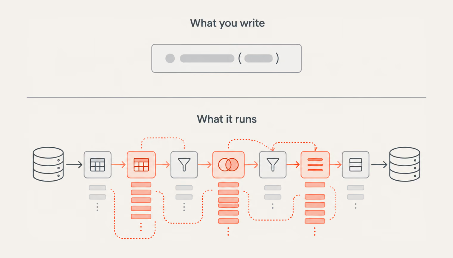
That moment leaves three ways forward: stay with the ORM, move to a query builder, or drop to raw SQL on the paths that hurt. Which one pays off depends on numbers rather than preference — how much speed each layer buys, and what it costs in development time. This guide puts the three head to head on real PostgreSQL benchmarks across Node.js, Python, and Java, then turns the results into a rule for which layer to reach for and when.

{{banner}}

Executive summary

For a quick orientation before the detailed numbers, these are the headline findings — where each layer’s strength lies and how the three compare at a glance:

• Raw SQL usually wins on raw speed. When latency is the whole game, hand-written SQL is hard to beat.
• Query builders are often the most balanced choice. They trade a little speed for a lot of control and maintainability.
• ORMs still lead on delivery speed. For ordinary business logic, they get features shipped fastest.
• A hybrid approach tends to hold up best long-term. The choice is a per-workload decision, and treating any one layer as the only right answer usually leaves performance or velocity on the table.

The one line worth keeping from all of it: optimize for engineering throughput first, then fix the measured bottlenecks with the sharper tool.

Benchmark setup

Every result below comes from the same controlled setup, so the comparisons are like-for-like:

A few things worth knowing about how the numbers were produced:

• Each access method ran against its own separately seeded but identical PostgreSQL dataset.
• The measurements are average latency, p95 latency, and throughput per operation.
• These are runtime figures from a local setup, so treat them as relative rather than absolute — both the exact milliseconds and the gaps between tools may shift in cloud or production environments.

Query by query: the same operation through each layer

Aggregate scores show the shape of things, and the sharper question is how one specific query performs when written three different ways. Each block below runs the same logical operation through pure SQL (pg), a query builder (Knex), and an ORM (Sequelize, TypeORM, or Prisma), so the difference is the access layer.

selectById

The simplest case — fetch one row by primary key. In pure SQL:

SELECT id, email, age, city, created_at
FROM users
WHERE id = $1;

Knex expresses it with a bit more ceremony, but the same intent:

await knex("users")
  .select("id", "email", "age", "city", "created_at")
  .where({ id })
  .first();

Run it a few thousand times, and the layers sort themselves out:

On a plain key lookup, the layers line up exactly as you’d expect: raw SQL fastest, the builder close behind, the ORMs trailing by the cost of their abstraction. The gap is real but small in absolute terms — a fraction of a millisecond per call.

filteredSelect

Now something with a bit more going on — a range filter, a sort, and a cap on rows. Here’s the SQL:

SELECT id, email, age, city, created_at
FROM users
WHERE age BETWEEN $1 AND $2
ORDER BY id DESC
LIMIT 20;

Knex chains the range, the ordering, and the limit into one fluent call:

await knex("users")
  .select("id", "email", "age", "city", "created_at")
  .whereBetween("age", [minAge, maxAge])
  .orderBy("id", "desc")
  .limit(20);

Running the same range query a few thousand times through each layer gives the following numbers:

This one upends the ordering: Prisma comes out ahead of raw SQL in this run, showing that an ORM can still outperform a lower-level access layer on a specific query shape.

aggregateGroupBy

This read query is the heaviest: count the users in each city and return the ten largest. It’s the kind of query that powers a dashboard, and the kind where the access layer’s overhead starts to matter. The query itself is straightforward SQL — a grouped count, sorted and capped:

SELECT city, COUNT(*) AS c
FROM users
GROUP BY city
ORDER BY c DESC
LIMIT 10;

Knex maps the grouping and count onto its builder methods almost one-to-one:

await knex("users")
  .select("city")
  .count("id as c")
  .groupBy("city")
  .orderBy("c", "desc")
  .limit(10);

Grouped work reshuffles the standings again:

Raw SQL is back on top here, but the more telling result is second place: TypeORM edges out Knex and the other ORMs. On this grouped query, TypeORM also shows that the ordering between abstractions can shift with the query shape.

updateById

The one write operation in this group: change a single user’s city by ID. In SQL, it’s about as small as a statement gets:

UPDATE users
SET city = $1
WHERE id = $2;

Knex collapses it to a single line:

await knex("users").where({ id }).update({ city });

Under load, the write ordering looks like this:

The ordering matches the simple key lookup — raw SQL fastest, the builder and TypeORM close behind, Prisma trailing furthest on this shape. For a single-row write, the abstraction cost is small in absolute terms but consistent.

Python results (avg ms)

The benchmark runs seven operations against each layer — a full CRUD set (insert, select, filtered select, update, delete), plus a grouped aggregate and a batch insert, chosen to cover the read, write, and bulk patterns a real app actually hits. Three of them are worth walking through in code, since they show the clearest contrasts between SQLAlchemy as the ORM, PyPika as the builder, and psycopg as the raw driver. The full seven land in the summary at the end.

selectById

The single-row lookup, in psycopg’s raw SQL:

SELECT id, email, age, city, created_at
FROM users
WHERE id = %s;

PyPika builds the same statement through its fluent API, then hands the rendered SQL to the cursor:

query = (
    Query.from_(users)
    .select(users.id, users.email, users.age, users.city, users.created_at)
    .where(users.id == user_id)
)
cur.execute(str(query))

SQLAlchemy reduces it to a single call, since fetching by primary key is what an ORM is built for:

with Session(engine) as s:
    user = s.get(User, user_id)

The timings track the Node result closely:

The raw driver leads clearly, the builder sits in the middle, and the ORM’s convenience shows up as latency — the same ordering as Node, with a wider spread.

aggregateGroupBy

The aggregate is the heaviest of the three — tally users per city, keep the top ten. Raw SQL states it plainly:

SELECT city, COUNT(*) AS c
FROM users
GROUP BY city
ORDER BY c DESC
LIMIT 10;

PyPika expresses the grouping and the count function through its builder:

query = (
    Query.from_(users)
    .select(users.city, fn.Count(users.id).as_("c"))
    .groupby(users.city)
    .orderby("c", order=Order.desc)
    .limit(10)
)
cur.execute(str(query))

SQLAlchemy builds the same aggregate as a Core statement:

stmt = (
    select(User.city, func.count(User.id).label("c"))
    .group_by(User.city)
    .order_by(text("c DESC"))
    .limit(10)
)
s.execute(stmt).all()

The grouping cost shows through in the timings:

Grouped work keeps the same ordering here, with SQLAlchemy showing a larger absolute gap from the raw driver than on the primary-key lookup.

updateById

The lone write in this set changes one user’s city. In raw SQL it’s a two-line statement:

UPDATE users
SET city = %s
WHERE id = %s;

PyPika composes the update and renders it for the cursor:

query = Query.update(users).set(users.city, city).where(users.id == user_id)
cur.execute(str(query))

SQLAlchemy here drops to a text statement with bound parameters, common for a targeted write:

s.execute(
    text("UPDATE users SET city = :city WHERE id = :id"),
    {"city": city, "id": user_id}
)
s.commit()

The single write lands each layer in the usual order:

The single-row write repeats the pattern: raw SQL fastest, the builder close, the ORM paying for its abstraction and session management.

Across the three queries, raw SQL wins each on latency, the builder trades a little speed for cleaner composition, and the ORM gives up latency for productivity on complex domain logic. The full run tells the same story with one exception worth its own line. On transactionBatchInsert, SQLAlchemy comes out well ahead of both, showing that an ORM can outperform lower-level options on a specific write path when its execution pattern fits the workload well.

A well-designed ORM write path can beat hand-rolled SQL on bulk work — which is why SQLAlchemy stays a sensible default for maintainable systems, psycopg remains the tool for optimized reads and write hotspots, and PyPika earns its place when composing complex queries dynamically matters more than mapping entities.

The fastest layer depends on the job, and sometimes the abstraction is the shortcut.

All seven operations side by side, including the four not walked through above:

Java results (avg ms)

Java pits JDBC as the raw driver against jOOQ as the builder and Hibernate as the ORM. The same representative queries, side by side — and this is where the benchmark stops agreeing with itself across languages.

selectById

Fetching one row by primary key is the barest test there is. JDBC writes it as plain parameterized SQL:

SELECT id, email, age, city, created_at
FROM users
WHERE id = ?;

jOOQ expresses it through a type-safe DSL, where every column and table is a generated Java object the compiler checks:

dsl.select(id, email, age, city, createdAt)
   .from(users)
   .where(id.eq(userId))
   .fetch();

Hibernate resolves the same lookup in one transactional call:

sessionFactory.inTransaction(session ->
    session.find(UserEntity.class, (long) userId));

On the simplest query, the layers separate the hardest:

JDBC clears seven thousand operations a second — roughly three times jOOQ and five times Hibernate. In this run, the relative gap is especially large on this simple primary-key lookup.

filteredSelect

A range filter with a sort and a limit adds more work to the query, starting with the raw SQL:

SELECT id, email, age, city, created_at
FROM users
WHERE age BETWEEN ? AND ?
ORDER BY id DESC
LIMIT 20;

jOOQ chains the filter and ordering with its builder methods, type-checked end to end:

dsl.select(id, email, age, city, createdAt)
   .from(users)
   .where(age.between(minAge, maxAge))
   .orderBy(id.desc())
   .limit(20)
   .fetch();

Hibernate reaches for HQL, its own query language written over the entity model:

session.createSelectionQuery(
    "from UserEntity u where u.age between :a and :b order by u.id desc",
    UserEntity.class)
    .setParameter("a", minAge)
    .setParameter("b", maxAge)
    .setMaxResults(20)
    .getResultList();

The heavier query tightens the field, exactly as predicted:

jOOQ closes some of the gap with JDBC on this heavier query, while Hibernate still trails both. In this run, the differences between the three layers are smaller than on the simple primary-key lookup, which suggests that access-layer overhead matters differently depending on the query shape and the amount of work the database is doing.

transactionBatchInsert

The batch write is the query that breaks the pattern, and it deserves a close look. JDBC feeds many rows through one prepared statement:

connection.setAutoCommit(false);
PreparedStatement ps = connection.prepareStatement(
    "INSERT INTO users (email, age, city, created_at) VALUES (?, ?, ?, ?)"
);
// addBatch() in a loop, then executeBatch() + commit()

jOOQ runs each insert on its own inside a single transaction:

c.setAutoCommit(false);
for (/* each row */) {
    dsl.insertInto(users).columns(email, age, city, createdAt)
       .values(emailV, ageV, cityV, createdAtV)
       .execute();
}
c.commit();

Hibernate persists each entity through the session:

sessionFactory.inTransaction(session -> {
    for (/* each entity */) {
        session.persist(entity);
    }
});

The margin is the widest in the whole benchmark:

JDBC runs about five times faster here, with its explicit batching avoiding much of the per-row execution overhead seen in the other two implementations. The telling part is cross-language: in Python, the ORM won this same operation, while JDBC leads decisively here.

Same operation, opposite winner — which is why “ORMs are slow at bulk writes” holds only until you measure your own stack. JDBC’s lead here also dwarfs pg’s in Node, showing how much the payoff from a lower-level access layer can vary across runtimes and implementations.

The full run, all seven operations, confirms JDBC’s near-total sweep:

Cross-language winners

Line the three languages up against each other, and the ceiling is almost always the same stack: Java on raw JDBC, fastest on six of the seven operations. Only the grouped aggregate goes elsewhere, to Python’s psycopg. The broader pattern still favors raw drivers: they win most operations across the three ecosystems. But the exceptions matter — Prisma leads one Node.js query, and SQLAlchemy wins the Python batch insert.

Hand-written SQL on a thin driver sets the speed ceiling in most of these benchmarks, while abstraction layers trade some of that speed for other benefits. Two charts show the shape of that gap more clearly than the numbers can. On a simple lookup, the raw drivers across all three languages cluster close together, and even the ORMs aren’t far behind:

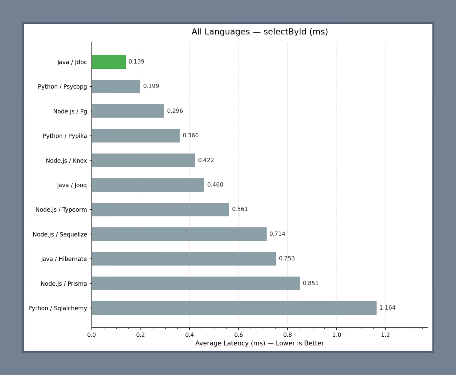
On a simple lookup, the gap between raw SQL and the ORM stays narrow in every language. On a batch insert, the same comparison breaks wide open — the spread multiplies and the languages diverge sharply, with Java’s JDBC batching far ahead of everything else:

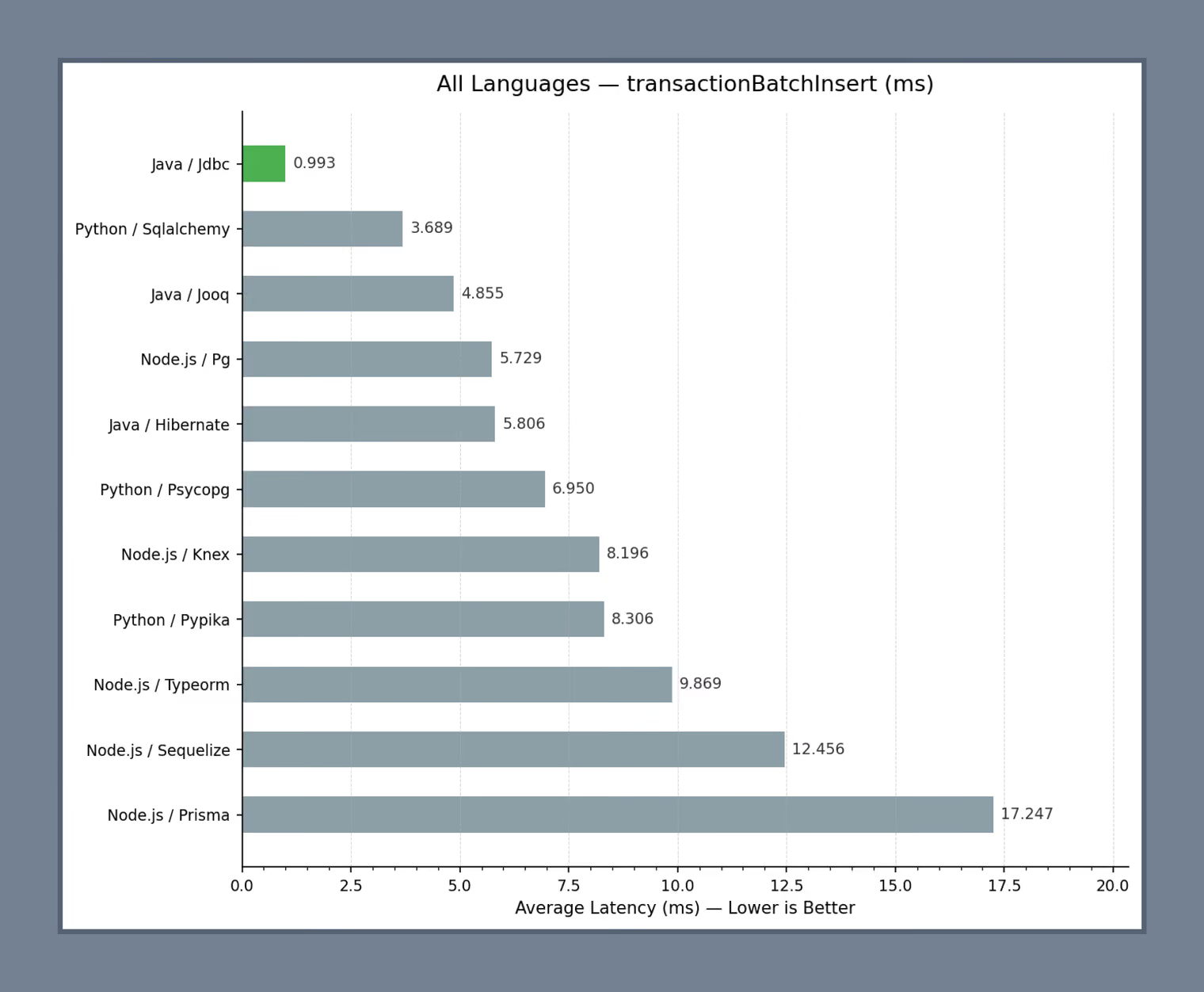
On a batch insert, the gap between layers widens sharply, and it differs by language. Together, the two charts show how much the impact of the access layer can change with the workload.

Choosing the right layer for the job

The benchmarks narrow the field, but the right choice depends on your situation more than on any single number. Four questions settle most of it:

1. Is the bottleneck engineering speed or database latency?
2. Are the queries mostly standard CRUD, or dynamic and analytical?
3. Does the team have strong SQL review discipline?
4. How costly is refactoring later in the product’s life?

The answers point toward one of the three layers.

Choose an ORM when:

• Feature delivery speed is the top priority.
• The workload is mostly CRUD and standard relations.
• The team’s SQL depth is mixed, and the abstraction keeps everyone productive.

Choose a query builder if:

• The queries involve complex filters, reporting, analytics, or dynamic composition.
• You want explicit control over the SQL while keeping composability and type safety, as with a Kysely database layer.
• Query evolution matters, and raw SQL strings would be harder to maintain than a builder.

Raw SQL earns its place when:

• A specific endpoint has been measured as a bottleneck.
• You need full control over the SQL shape and the execution plan.
• The team can hold the discipline that raw SQL demands — review, tests, profiling.

Where Prisma and TypeORM fit

The Node.js benchmark includes Sequelize, Prisma, and TypeORM, but the three take different approaches and suit different team preferences:

• Prisma puts a strong emphasis on developer experience — strong type safety, a clear schema-first workflow, and a natural fit for modern TypeScript teams. The trade-offs to watch: some advanced SQL patterns still need a raw-query escape hatch, and query behavior should be profiled under real load rather than trusted.
• TypeORM is the more flexible of the two, supporting both Data Mapper and Active Record patterns, with a rich ecosystem and broad driver support — a good fit for teams that want classic entity-based architecture. It asks for more governance in return: relation loading and query behavior need active review, and like any ORM, it can hide performance problems when SQL observability is weak.
• Sequelize, one of the benchmarked ORMs, remains a mature option with wide adoption, though its generated queries carry overhead on some paths.

The best ORM is the one your team can measure and control under real load.

Putting the three to work together

The benchmarks answer which layer is fastest. The harder question in a real codebase is how they coexist, and the answer is that they should. A mature data layer uses all three, each on the work it suits, with clear boundaries between them:

Where teams go wrong is picking one tool for everything and forcing it onto work it was never suited for.

What each layer looks like in place

An ORM handles a domain workflow cleanly — fetch the entity, change it, save it:

const user = await prisma.user.findUnique({ where: { id: userId } });
if (!user) throw new Error("User not found");
await prisma.user.update({ where: { id: userId }, data: { city: "Lviv" } });

A query builder shines in API development and other cases where the query is assembled dynamically, adding conditions only when they apply:

const q = knex("users").select("id", "email", "age", "city");
if (filters.minAge) q.where("age", ">=", filters.minAge);
if (filters.city) q.where("city", filters.city);
const rows = await q.orderBy("id", "desc").limit(50);

Raw SQL takes over on a measured hotspot, where full control over the query and its plan is worth the maintenance cost:

SELECT city, COUNT(*) AS c
FROM users
WHERE age BETWEEN $1 AND $2
GROUP BY city
ORDER BY c DESC
LIMIT 10;

The mistakes that undo it

A few habits reliably turn this arrangement back into a problem:

• Declaring “the ORM is slow” without measuring. It leads to expensive rewrites that fix nothing, because the real bottleneck was somewhere else.
• Reaching for raw SQL everywhere. It buys speed the app doesn’t need and pays for it in maintenance and onboarding costs.
• Mixing styles inconsistently across modules. When every module accesses data differently, debugging and ownership get murky.
• Optimizing average latency alone. Incidents live in the tail, so p95 and p99 are what decide whether the system holds under load.

Keeping it honest in production

The arrangement holds only with the instrumentation to see when it slips. A short standing checklist covers most of it:

• Log query durations for slow-path analysis.
• Track average, p95, and throughput on critical endpoints.
• Run EXPLAIN ANALYZE on the expensive queries.
• Add benchmark regressions to CI for core operations.
• Keep the data-access style consistent within each module.

Two habits keep the arrangement honest over time: run EXPLAIN ANALYZE on the queries that surface as expensive, and add benchmark regressions to CI so a slowdown on a core operation gets caught before it ships.

The choice changes with the workload

The benchmarks point to a simpler conclusion than the usual ORM-versus-raw-SQL debate suggests. Raw SQL wins most of the measured operations, but not all of them, and the exceptions matter. An ORM can come out ahead on a specific write path, while a query builder may offer enough control without giving up the structure a team relies on.

That makes the choice less about picking one layer and more about knowing when to use each one. In software product development, start with the option that keeps the work moving, measure where performance actually slips, and reach for more control only where the data shows it is needed. The real advantage is not committing to one tool. It is keeping the data-access layer flexible enough to change with the workload.

{{banner-2}}